bang for your bits: lossless neural compression (part 1)

Maybe it's just me, but whenever I think about compression the first thing that comes to mind is lossy compression. We give up some quality for smaller file sizes, happens all the time. Whenever I do something like that, I always have the original file around, just so I don't keep losing information (like the concept of a film negative).

Lossless compression is primarily concerned with representing data with as few bits as possible so that no information is lost.

What confused me at first was my (incorrect) idea that compression = information lost. This isn't the case. Consider trying to store a colour image. What's the easiest way to do this? We could use an array of pixels, with 3 values (red, green, blue) for each pixel. This seems workable, until you imagine storing this image:

It seems like overkill to store every white pixel as (255, 255, 255), over and over.¹

Such is why lossless compression exists — most data has redundancies we can get rid of without losing information. A good example is a .zip file — you zip a folder to make it smaller (take fewer bits; compression), and when you unzip it your files are exactly the same (perfect reconstruction; lossless).²

Now let's abstract some stuff away. Our problem is trying to encode a sequence of symbols called a message into a sequence of bits.³ Let's say the space of possible symbols (alphabet) is $\mathcal{A}$. We're going to use symbol codes: every symbol $a\in \mathcal{A}$ will have a bitstring (codeword) assigned to it. Like Morse code! Or ASCII!

Let's try the obvious solution first. Say $||\mathcal{A}|| = N$ (there are $N$ possible symbols, $N$ letters in our alphabet). What if we just use $\log_2 N$ (rounded up) bits, and each possible bitstring is a letter? For example, in the case of the lowercase latin alphabet, $N=26$, so we would need 5 bits, and assign the possible 5-bit codes in order? a=00000, b=00001, c=00010, d=00011, ..., x=10111, y=11000, z=11001

Like our image example, this seems workable until you realize that q uses the exact same amount of space as e. It's like if every letter in Scrabble had the same value. Intuitively, since e is much more frequently used, we'd want a short codeword for it. Similarly, since z is less frequently used, we don't care too much if it has a longer codeword for it.

Take a moment to formalize this intuition. Intuitively, we're looking at frequencies: which symbols are likelier to appear in a given message. We can introduce ideas about probability and use that to find our optimal coding scheme. We won't have every possible message beforehand, and thus we need to model messages with probability.

Formally, let $X$ be a discrete random variable (finitely many possibilities) with probability distribution (how likely each outcome is) $P$. A message is a sequence of outcomes of $X$. We wish to find a prefix-free code (no codeword is a prefix of another, to avoid ambiguous cases like e=0, x=01) such that higher probability outcomes of $X$ have shorter codewords.

codewords

For now, assume that we know exactly what $P$ is. Later, we'll see how we can use neural networks to approximate $P$ when this assumption isn't true.

Let's take a moment to characterize what we would expect of a solution given some distributions $P$. If $P$ is uniform, every symbol is equally likely to come up, so our naive solution works pretty well. Since we probably won't have exactly power-of-2 symbols, we can drop some bits to make it optimal, but our expected codeword length is probably somewhere around $\log_2 N$ bits. Instead if we say $P$ is heavily biased towards two symbols and the rest basically never show up. Then our expected codeword length is somewhere around 1, since we can use 0 and 1 to encode the two most common symbols.

Here's the pièce de résistance: we can combine this with the notion of entropy, that is, the expected value of surprise. The core of information theory is defining information as measuring surprise. A more surprising result gives us more information. The entropy measures the expected value of surprise for $X$. Each time we sample $X$ (roll the dice, flip the coin, draw the ticket, pick the number, whatever), how surprised do we expect to be? Or: how much information do we expect? Or: how much do we expect to cut our sample space?

The formula for entropy is this:

where $\mathbb{E}$ represents expected value. The thing that links entropy to our compression problem is the notion that more information needs more bits.

Let's take our earlier case where $P$ favours two symbols equally and ignores all the rest. What is the entropy of $X$? Well,

and we also happened to need only 1 bit to compress our message.

Hmm.

Intuitively, the expected amount of information (entropy, $H$) should be connected to how many bits we need to represent it. This is Shannon's source coding theorem, basically the fundamental theorem of information theory. The formal proof is a little complicated, but I'll write about it separately.

So we've now formulated our problem and established its connection to information theory. Now let's go over an implementation: Huffman coding.

Originally, this was going to be two parts: formulation of the problem, then solving it. It turns out the algorithm is beautifully simple, so this feels like a footnote. It's not, really.

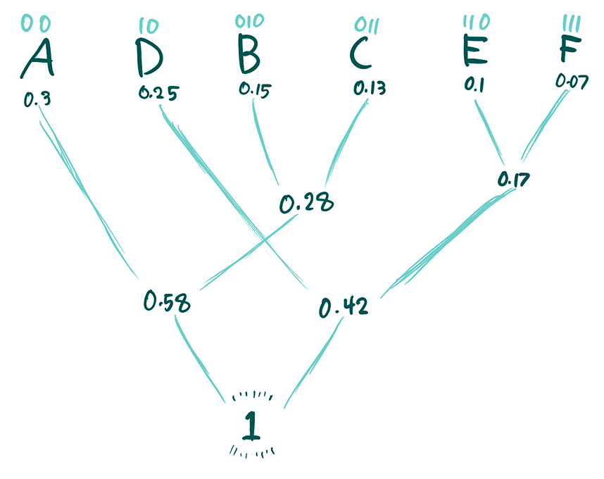
We have our probabilities for every symbol $x\in \mathcal{X}$. These will be the leaves of the tree we'll use to encode. Recursively merge the two nodes (leaves are also nodes) with the lowest probability, with lower probability on the right. Continue until you have the node with probability $1$. To encode a symbol, walk down the tree until you get to a symbol, 0 if you go left, 1 if you go right. Once you get to your symbol, you'll have a unique codeword that's prefix-free for that symbol.

Let's go back to our definition to see if this works.

1. Lossless: obviously every leaf has a unique path to it, so it has a unique codeword. Also, every codeword will reach a leaf at some point. Thus we can always retrieve our symbols from our code without any error.
2. Compression: our tree was formed by merging nodes with the smallest probabilities, so leaves with low probabilities are farther away from the root and thus have longer codewords. Leaves with higher probabilities avoid being merged for longer, so they have shorter codewords. This should make sense intuitively, but I have a formal proof in the footnotes. If you want to prove it yourself, a hint: "think local."

Huffman coding always finds the optimal prefix-free symbol coding scheme. But because of the discrete nature of bits, it still misses out a bit in extreme cases. It assigns a codeword of length at most $\lceil{-\log_2 P(a)\rceil}$ to $a$. Log-probabilities usualy aren't integers, so the discretization inherent in the ceiling function makes us lose out. For example, it still takes one bit to encode a symbol with 99% probability, even though it carries much less than one bit of information (its entropy is close to 0).

We can't use a fractional number of bits for one symbol. But maybe we can expand our purview from going symbol by symbol, aggregating the fractional bits across a whole message? If the symbol $A$ has probability 99%, then the message $A\dots A(70)$ carries about 1 bit of information ($-\log_2 (0.99)^{70} =-70\log_2 0.99 \approx 1.01$), so we might be able to save about 69 bits — significant savings!

significant savings

One way of doing so is a method called arithmetic coding. The idea is that we're going to split up a unit interval ($[0, 1]$) based on the probabilities of symbols occurring. Taking the general interval $[a, b)$, we're going to create sub-intervals sized proportionally to the symbol probabilities. We iteratively do this until we get to the end of the message. The intervals get smaller as we go — once we're done, we can pick any real number in our interval to represent our message.

This essentially allows us to allocate fractional bits as we go, removing the mandatory 1-bit overhead that Huffman coding requires. We can't represent arbitrary real numbers in finitely many bits, so instead we can quantize to the nearest binary fraction based on the smallest length. For example, if $l$ is the length of the smallest interval,

• $l \in [0.5, 1)$, quantize to $0.0_2, 0.1_2$ (1 bit)
• $l \in [0.25, 0.5)$, quantize to $0.00_2, 0.01_2, 0.10_2, 0.11_2$ (2 bits)
• $l \in [0.125, 0.25)$, use $0.000_2, 0.001_2, \dots, 0.111_2$ (3 bits)
• and so on,

The shorter the interval, the more binary digits we need to get a fraction in that interval (including trailing 0's), but also the less likely that sequence is. Extend this pattern, and you get that the minimum number of bits we need to represent the message is, in general, $\lceil{-\log_2 (l_N)\rceil}$. That looks familiar!

Arithmetic coding reaches the theoretical bound on compression (the entropy of the sequence) and the quantization (ceiling function) is applied to the entire message — our overhead is amortized and becomes less and less significant the longer our sequence.

In our idealized world, we have as many bits as we want. We can't represent arbitrary real numbers in the finitely many bits we have, so we have to handle rounding error. In particular, the length of our interval approaches 0 as our message continues; probabilities multiply and become small quickly, so we quickly run into precision issues.

Arithmetic coding thus typically has some extra bits ⁴ to make it easier (and possible) to implement. First, a process called renormalization is used — this basically corresponds to a "zooming in" after each step, rescaling our interval so that it matches our original interval size. Second, instead of using fractions in the unit interval, it's typically easier to deal with integers. Essentially, if we were had 64 bits of precision for the fractional parts, we can use 64-bit integers instead. That means that, conceptually, we'll deal with ex. 256 integer values rather than 256 binary fractions.

There are other implementation concerns too, but I'll leave it to this book to deal with them.

Let's revisit our definition. We've covered compression already — arithmetic coding gets to ~ our entropy limit on compression. As for lossless, ... ah. There's also the problem of knowing where to stop. We need an EOF character. Another 1 bit overhead! Not too big a deal. Other than that, we can always just retrace the steps of the compressor to decompress the message.

There's another lossless compression algorithm in the books. Since this reaches pretty close to the entropy coding limit, to compress further we need to find some other redundancies to eliminate. So far, we've been treating symbols as independent and identically distributed. But that's obviously not true. If you look at q's in the English language, they're almost always followed by u's.⁵

Somehow, we want to understand what messages are likelier than others beyond just what letters that contain, and it's not immediately clear how we could set up an explicit set of rules to do that.

Hm.

That seems like AI could help.

But I'll save that for the next post. ⁶

Thanks to one of my mentors for recommending this neural compression workshop and for sharing this paper, which catalyzed a reading trail that led me here.

Footnotes

1. Whenever tackling a problem, it's always good to think of the "dumbest" possible solution first and see where it gets us. If nothing else, at least it lets us understand what the heck is going on. ↩

2. Both .zip and .png uses lossless compression schemes, and in fact they use the same compression algorithm (called DEFLATE). That's why if you try to zip a png you'll barely save any storage. Try it! ↩

3. Italicizing bits is a little strange here, but I want to emphasize that we can only use 0s or 1s. ↩

4. in the sense of pieces, not, you know, extra bits. I'm known for being funny by the way. ↩

5. Calling back to that scrabble analogy, apparently scrabble tournament competitors memorize words with q's and no u's so they can always play their q. ↩

6. A preview: autoregressive models are widely used for learning conditional distributions for sequential data, fitting perfectly with arithmetic coding. Both deal with probabilities symbol by symbol, and both operate in a particular order (a queue). We can use an autoregressive model (e.g. and RNN) to better estimate the probability of each symbol, taking into account the dependencies between characters. It's limited, as autoregressive modelling often is, by the sequential constraints limiting decoding speed. More about this, latent variable models and bits-back coding in a future post:) ↩